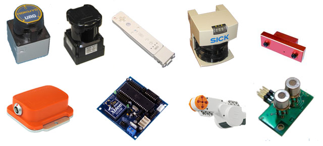
This is a list I compiled of sensors for robots that already have support in ROS2. As you can see, there are just a few, and most of the drivers are outdated and for old ROS2 distributions. It may require some adaptation work to use these drivers for a modern ROS2 distribution.
If you are a sensor company or a ROS Developer, and you provide support for a sensor in ROS2, please let me know so I can update the list with your work.
If you are interested in robotics, you must have heard of ROS (Robot Operating System). ROS is now very popular among roboticists. Researchers, hobbyists, and even robotics companies are using it, promoting it. and supporting it. But what is ROS? How did ROS reach its current state as a robotics standard? Why is ROS becoming a must-have skill for robotics practitioners? In this article, we will reveal the answers to these questions.
Keep on reading to understand ROS, or jump ahead to the section that interests you most.
Before we understand what ROS is, let me introduce you to ROS with a short history of how it started, the main reasons behind it, and its current status.
The Stanford Period
Similar frameworks at the time
Switching gears
Willow Garage takes the lead
Under the Open Source Robotics Foundation umbrella
ROS 2.0
Recent movements in the ROS ecosystem
The Stanford Period
ROS started as a personal project of Keenan Wyrobek and Eric Berger while at Stanford, as an attempt to remove the reinventing-the-wheel situation from which robotics was suffering. These two guys were worried about the most common problem of robotics at the time:
too much time dedicated to re-implementing the software infrastructure required to build complex robotics algorithms (basically, drivers to the sensors and actuators, and communications between different programs inside the same robot)
too little time dedicated to actually building intelligent robotics programs that were based on that infrastructure.
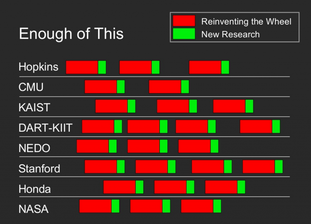
Even inside the same organization, the re-invention of the drivers and communication systems was re-implemented for each new project. This situation was beautifully expressed by Keenan and Eric in one of their slides used to pitch investors.
Most of the time spent in robotics was reinventing the wheel (slide from Eric and Keenan pitch deck)
In order to attack that problem, Eric and Keenan created a program at Stanford called the Stanford Personal Robotics Program in 2006, with the aim to build a framework that allowed processes to communicate with each other, plus some tools to help create code on top of that. All that framework was supposed to be used to create code for a robot they would also build, the Personal Robot, as a test bed and example to others. They would build 10 of those robots and provide them to universities so that they could develop software based on their framework.
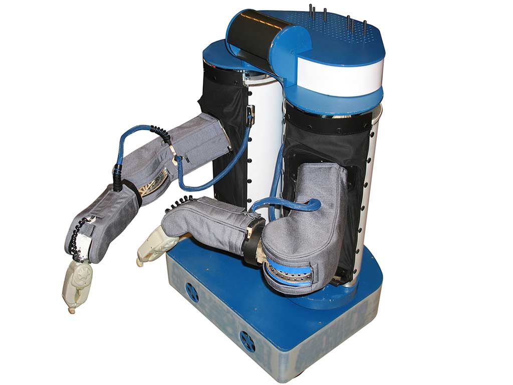
NOTE: People more versed in ROS will recognize the precursors of ROS-comm libraries and the Rviz, rqt_tools and the like of current modern ROS distributions. Also, the Personal Robot was the precursor to the famous PR2 robot.
PR1 robot, picture by IEEE Spectrum
Similar frameworks at the time
The idea of such a system for robotics was not new. Actually, there were some other related projects already available for the robotics community: Player/Stage, one of the most famous in the line of open source, and URBI in the line of proprietary systems. Even Open-R, the system developed by Sony, which powered the early Aibo robots of 1999, was a system created to prevent that problem (a shame that Sony cancelled that project, as they could have become the leaders by now. Ironically, this year, Sony launched a new version of the Aibo robot… which runs ROS inside!). Finally, another similar system developed in Europe was YARP.
Actually, one of the leaders of the Player/Stage research project was Brian Gerkey, who later went to Willow Garage to develop ROS, and is now the CEO of Open Robotics, the company behind the development of ROS at present. On its side, URBI was a professional system led by Jean-Christoph Baillie, which worked very well, but could not compete with ROS, which was free.
The fastest readers will jump to the point that URBI was not free. Actually, it was quite expensive. Was the price what killed URBI? I don’t think so. In my opinion, what killed URBI was the lack of community. It takes some time to build a community, but once you have it, it acts like changing gears. URBI could not build a community because it relied on an (expensive) paid fee. That made it so that only people that could buy it were accessing the framework. That limits the amount of community you can create. It is true that ROS was free. But that is not the reason (many products that are free fail). The reason is that they built a community. Being free was just a strategy to build that community.
Switching gears
While at Stanford, Keenan and Eric received $50k of funding and used it to build a PR robot and a demo of what their actual project was. However, they realized that in order to build a really universal system and to provide those robots to the research groups, they would need additional funding. So they started to pitch investors.
At some point around 2008, Keenan and Eric met with Scott Hassan, investor and the founder of Willow Garage, a research center with a focus on robotics products. Scott found their idea so interesting that he decided to fund it and start a Personal Robotics Program inside Willow Garage with them. The Robot Operating System was born, and the PR2 robot with it. Actually, the ROS project became so important that all the other projects of Willow Garage were discarded and Willow Garage concentrated only on the development and spread of ROS.
Willow Garage takes the lead
ROS was developed at Willow Garage over the course of 6 years, until Willow shut down, back in 2014. During that time, many advancements in the project were made. It was this push during the Willow time that skyrocketed its popularity. It was also during that time that I acknowledged its existence (I started with ROS C-turtle in 2010) and decided to switch from Player/Stage (the framework I was using at that time) to ROS, even if I was in love with Player/Stage (I don’t miss you because ROS is so much better in all aspects… sorry, Player/Stage, it’s not me, it’s you).
In 2009, the first distribution of ROS was released: ROS Mango Tango, also called ROS 0.4. As you can see, the name of the first release had nothing to do with the current naming convention (for unknown reasons to this author). The release 1.0 of that distribution was launched almost a year later in 2010. From that point, the ROS team decided to name the distributions after turtle types. Hence, the following distributions and release dates were done:
In 2009, they built a second version of the Personal Robot, the PR2
In xxx, they launched ROS Answers, the channel to answer technical questions about ROS.
The first edition of the ROSCON was in 2012. The ROSCON became the official yearly conference for ROS developers.
In 2010, they built 11 PR2 robots and provided them to 11 universities for robotics software development using ROS (the original idea of Eric and Keenan). At that point, the PR2 robot was for sale, so anybody in the world could buy one (if enough money was available ;-)).
Simulation started to become very important. More precisely, 3D simulation. That is why the team decided to incorporate Gazebo, the 3D robotics simulator from the Player/Stage project, into ROS. Gazebo became the default 3D simulator for ROS.
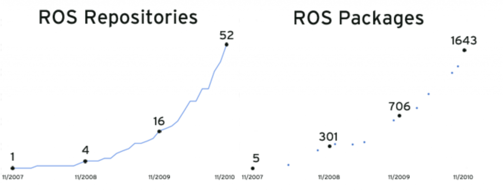
As ROS was evolving, all the metrics of ROS were skyrocketing. The number of repositories, the number of packages provided, and of course, the number of universities using it and of companies putting it into their products.
Evolution of ROS in the early days (picture from Willow Garage)
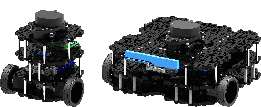
Another important event that increased the size of the ROS community was when, in 2011, Willow Garage announced the release of the Turtlebot robot, the most famous robot for ROS developers. Even if PR2 was the intended robot for testing and developing with ROS, its complexity and high price made it non-viable for most researchers. Instead, the Turtlebot was a simple and cheap robot that allowed anybody to experiment with the basics of robotics and ROS. It quickly became a big hit, and is used even today, in its Turtlebot2 and Turtlebot 3 versions.
I remember when we received the news that Willow Garage was closing. I was working at Pal Robotics at the time. We at Pal Robotics were all very worried. What would happen with ROS? After all, we had changed a lot of our code to be working with ROS. We removed previous libraries like Karto for navigation (Karto is software for robot navigation, which at present is free, but at that time, we had to pay for a license to use it as the main SLAM and path planning algorithms of our robots).
The idea was that the newly created Open Source Robotics Foundation would take the lead in ROS development. And many of the employees were absorbed by Suitable Technologies (one of the spin-offs created from Willow Garage, which ironically does not use ROS for their products ;-)). The customer support for all the PR2 robots was absorbed by another important company, Clearpath Robotics.
Under the Open Source Robotics Foundation umbrella
Under the new legal structure of the OSRF, ROS continued to develop and release new distributions.
The reports created after each year are publicly available here under the tag ROS Metrics.
Having reached this point, it is important to state that the last distribution of ROS will be released in 2020. It is called ROS Noetic, which will be based on Python 3, instead of Python 2 as all the previous ones were. From that date, no more ROS 1 distributions will be released, and the full development will be taken for ROS 2.
Around 2015, the deficiencies of ROS for commercial products were manifesting very clearly. Single point of failure (the roscore), lack of security, and no real-time support were some of the main deficiencies that companies argued for not supporting ROS in their products. However, it was clear that, if ROS had to become the standard for robotics, it had to reach the industrial sector with a stronger voice than that of the few pioneer companies already shipping ROS in their products.
In order to overcome that point, the OSRF took the effort to create ROS 2.0.
ROS 2.0 had already reached its fourth distribution in June 2019 with the release of Dashing Diademata.
Recent movements in the ROS ecosystem
In 2017, the Open Source Robotics Foundation changed its name to Open Robotics, in order to become more of a company than a foundation, even if the foundation branch still exists (some explanation about it can be found in this post and in this interview with Tully Foote).
Recently, Open Robotics has opened a new facility in Singapore and established a collaboration with the government there for development.
Local ROS conferences have been launched:
ROSCON France
ROSCON Japan
In the last few months, big players like Amazon, Google, and Microsoft have started to show interest in the system, and show support for ROS.
That is definitely a sign that ROS is in good health (I would say in better than ever) and that it has a bright future in front of it. Sure, many problems will arise (like, for example, the current problem of creating a last ROS 1 distribution based on Python 3), but I’m 100% sure that we, and by we I mean the whole ROS community, will solve them and build on them.
What is ROS?
Why are there not enough developers for robotics?
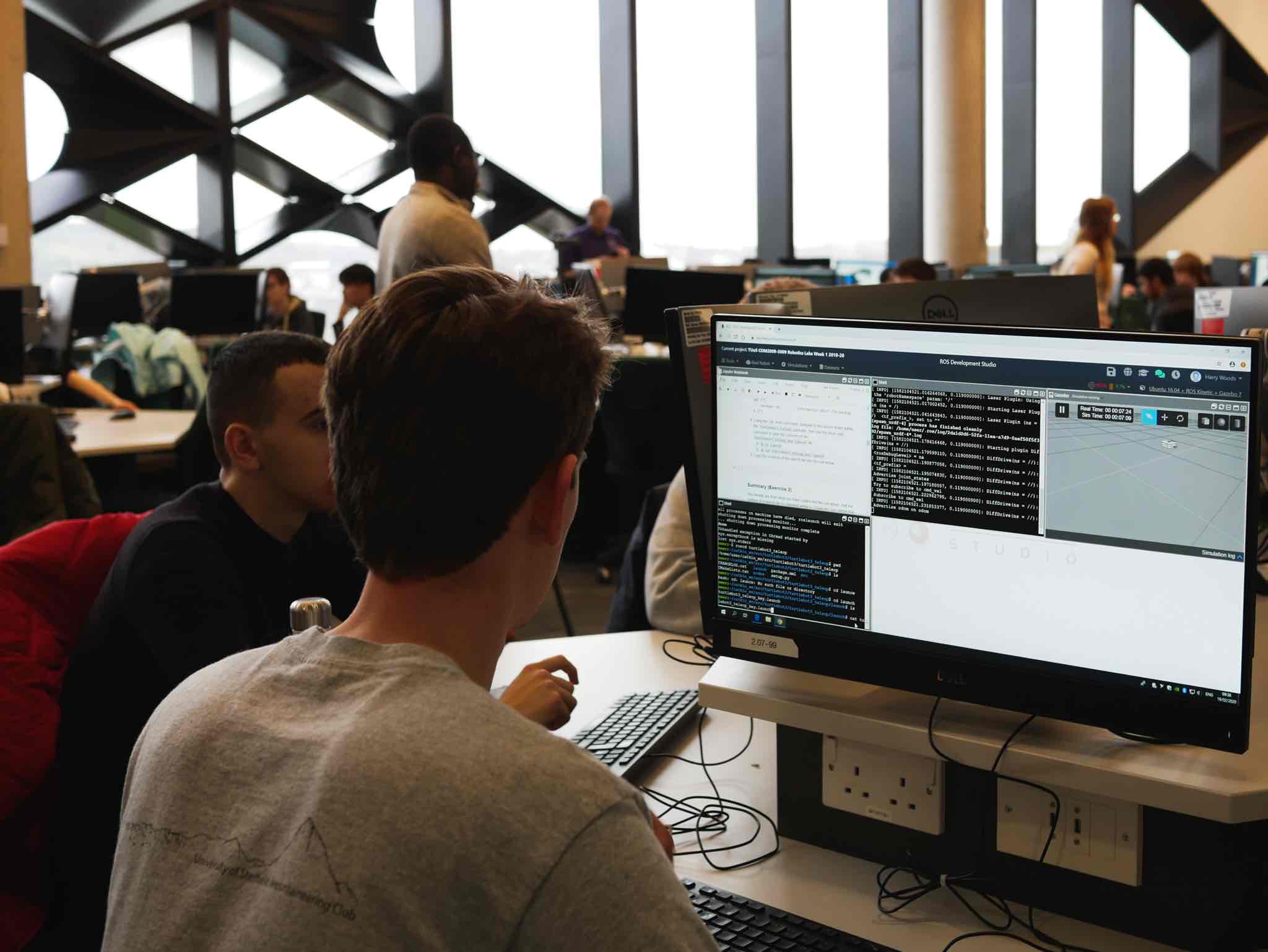
Roboticists programming robots
What is the robot ROS API?
What is ROS anyway?
ROS for service robots
ROS for industrial robots
ROS for agricultural robots
A story of software & hardware: why are there not enough developers for robotics?
In general, software developers do not like to deal with hardware. It is very likely that you are a software developer and never thought about entering into the robotics field. You probably think that by programming for robots, you would have to know about electronics, and maybe even mechanics. You probably think that hardware and software are too coupled in robots, that you cannot touch one without touching the other. And sometimes, it is true…
About 10 years ago, we had to develop a navigation system for a robot. However, our navigation program was not working at all. We thought that it was something wrong with the program, but after extensive review and testing in simulations, we found that it actually was a problem with the electronics of the laser scanner that we used to localize the robot. In order to find that error, we had to go to the basics and find where the problem within the physical laser was. For that, we needed to mess with the electronics. We had to take the laser out of the robot, put it on the table, and start experimenting. Different voltages, different interruptions to the power, all in order to try to reproduce the effect in a controlled environment. That is a lot of interaction with the hardware.
That interaction with the hardware is something that many software developers don’t like. After all, they decided to become software developers, not hardware developers!!
Roboticists programming robots
Due to this, the programming of robots has been done by roboticists, who are the people that build the robots. Maybe some of the roboticists were not directly involved in the creation of the robot, but they definitely have no problem getting into the hardware and trying to fix hardware problems in order to make their programs work.
But let’s face it, most roboticists are not as good at programming as software developers are. That is why robotics could benefit so much from having lots of expert programmers coming to the field.
The good news is that getting developers into the field is easier than ever. Thanks to the Robot Operating System, ROS, you can completely abstract the hardware from the software, so you can program a robot just by knowing the robot’s ROS API and having a simulation for testing. By using the ROS API, you can forget about the hardware and just concentrate on the software that makes the robot do what you want.
What is the robot ROS API?
The ROS API is the list of ROS topics, services, action servers, and messages that a given robot is providing to give access to its hardware, that is, sensors and actuators. If you are not familiar with ROS, you may not understand what those terms mean. But simply put in the developers’ language, topics/services/messages are like the software functions you can call on a robot to get data from the sensors or make the robot take action. It also includes the parameters you can pass on to those functions.
Most modern robot builders are providing off-the-shelf ROS APIs, for example, the ROS-Components shop that provides all its hardware running with a ROS API.
If the robot you want to work with does not run ROS, you can still make the robot work with ROS by ROSifying it. To ROSify means to adapt your robot to work with ROS. ROSifying a robot usually requires knowledge to access the hardware. You need to learn how to communicate with the electronics that provide the sensor data or access the motors of the robot. In this series of ROS tutorials, we are not dealing with that subject because it gets out of scope for developers. But if you are interested in this topic, you can learn more about it in this Robot Creation Course.
What is ROS anyway?
ROS stands for Robot Operating System. Even if the name says so, ROS is not a real operating system since it goes on top of Linux Ubuntu (also on top of Mac, and recently, on top of Windows). ROS is a framework on top of the O.S. that allows it to abstract the hardware from the software. This means, you can think in terms of software for
all the hardware of the robot. And that is good news for you because this implies that you can actually create programs for robots without having to deal with the hardware. Yea!
ROS works on Linux Ubuntu or Linux Debian. Experimental support already exists for OSX, Gentoo, and a version for Windows is under way, but we really don’t recommend for you to use them yet unless you are an expert. Check this page for more information about how to use ROS on those systems.
ROS for service robots
ROS is becoming the standard in robotics programming, at least in the service robots sector. Initially, ROS started at universities, but quickly spread into the business world. Every day, more and more companies and startups are basing their businesses on ROS. Before ROS, every robot had to be programmed using the manufacturer’s own API. This means that if you changed robots, you had to start the entire software again, apart from having to learn the new API. Furthermore, you had to know a lot about how to interact with the electronics of the robot in order to understand how your program was doing. The situation was similar to that of computers in the 80s, when every computer had its own operating system and you had to create the same program for every type of computer. ROS is for robots like Windows is for PCs, or Android for phones. By having a ROSified robot, that is, a robot that runs on ROS, you can create programs that can be shared among different robots. You can build a navigation program, that is a program to make a robot move around without colliding, for a four-wheeled robot built by company A and then use the same exact code to move a two-wheeled robot built by company B… or even use it on a drone from company C, with minor modifications.
ROS for industrial robots
ROS is being used in many of the service robots that are created at present. On the other side, industrial robotics companies are still not completely convinced about using it, mainly because they will lose the power of having a proprietary system. However, four years ago, an international group called ROS-Industrial (https://rosindustrial.org/) was created, whose aim is to make industrial manufacturers of robots understand that ROS is for them, since they will be able to use all the software off-the-shelf that other people have created for other ROS robots.
ROS for agricultural robots
In the same vein as ROS-Industrial, ROS-Agriculture (http://rosagriculture.org/) is another international group that aims to introduce ROS for agriculture robots. I highly recommend that you follow this group if you are interested because they are a very motivated team that can do crazy things with several tons of machine, by using ROS. Check out, for instance, this video (https://youtu.be/obu_Ru2gDHk) about an autonomous tractor running ROS, built by Kyler Laird of the ROS Agriculture group.
Why ROS?
The question then is this: why has ROS emerged on top of all the other possible contestants? None of them is worse than ROS in terms of features. Actually, you can find some features in all the other middlewares that outperform ROS. If that is so, why or how has ROS achieved the status of becoming the standard?
A simple answer from my point of view: excellent learning tutorials and debugging tools.
Here is a video where Leila Takayama, early developer of ROS, explains when she realized that the key for ROS to be used worldwide would be to provide tools that simplify the reuse of ROS code. None of the other projects have such a set of clear and structured tutorials. Even less, those other middlewares provide debugging tools in their packages. Lacking those two essential points is preventing new people from using their middlewares (even if I understand why the developers of OROCOS and YARP for not providing it… who wants to write tutorials or build debugging tools… nobody! 😉 )
Additionally, it is not only about Tutorials and Debugging-Tools. ROS creators also managed to create a good system of managing packages. The result of that is that developers worldwide could use others’ packages (relatively) easily. This created an explosion in available ROS packages, providing almost anything off-the-shelf for your brand-new ROSified robot.
Now, the rate at which contributions to the ROS ecosystem are made is so fast that it makes ROS almost unstoppable in terms of growth. According to ABI Research, about 55% of the world’s robots will include a ROS package by 2024. This is an indication of the fact that in ten years, ROS has become a defacto robotics standard, in academia and increasingly in industry. More and more universities are teaching robotics with ROS. The ROS Curriculum For Campus project that we launched in 2018 has been used by hundreds of universities. It is easy to see why ROS has become a must-have skill in the CV of robotics practitioners.
How to start learning ROS
Now, if you are convinced about becoming a ROS developer 😉 then using this beginner’s guide, we can follow these five steps to successfully learn ROS:
In order to create ROS programs, you will need a C++ or Python code editor. In this chapter, we are going to show you a list of integrated environments for programming ROS with those languages.
In this post, we are going to show a way of creating a custom program to send desired positions with respect to the task space of the Open Manipulatorend effector.
There are many possibilities to program this robot. For the sake of simplicity, we will use a single service available to move the arm to a specific position.
Although, the step-by-step explanation will show you how to use everything this simulation provides.
Configuring the Environment
If you haven’t configured the environment from the previous ROSJect, please open it using this link.
Though if you prefer to learn how to configure the environment and the simulation from scratch, start from this post.
How to interact with the robot – Choosing a specific service
After having the simulation running, you need to launch the controller node. This node will provide the services that send references to the real robot or the simulation (in this case, it is the simulation).
Then, in another web shell, we are able to check the services available:
user:~$ rosservice list
We have many services available, let’s check the one we will use, which is /open_manipulator/goal_task_space_path_position_only.
In order to call for the service, we need to know its structure:
user:~$ rosservice type /open_manipulator/goal_task_space_path_position_only

open_manipulator_msgs/SetKinematicsPose
We have to deal with this kind of message: open_manipulator_msgs/SetKinematicsPose
Its structure is:
user:~$ rossrv show open_manipulator_msgs/SetKinematicsPose

string planning_group
string end_effector_name
open_manipulator_msgs/KinematicsPose kinematics_pose
  geometry_msgs/Pose pose
    geometry_msgs/Point position
      float64 x
      float64 y
      float64 z
    geometry_msgs/Quaternion orientation
      float64 x
      float64 y
      float64 z
      float64 w
  float64 max_accelerations_scaling_factor
  float64 max_velocity_scaling_factor
  float64 tolerance
float64 path_time
---
bool is_planned
Let’s code!
Certainly, we need a simple ROS node that will act as a service client. The basic structure goes below:
#!/usr/bin/env python

import sys
import rospy
from open_manipulator_msgs.srv import *

def set_position_client(x, y, z, time):
    ...

def usage():
    return "%s [x y z]"%sys.argv[0]

if __name__ == "__main__":

    if len(sys.argv) == 5:
        x = float(sys.argv[1])
        y = float(sys.argv[2])
        z = float(sys.argv[3])
        time = float(sys.argv[4])
    else:
        print usage()
        sys.exit(1)
    print "Requesting [%s, %s, %s]"%(x, y, z)
    response = set_position_client(x, y, z, time)
    print "[%s %s %s] returns [%s]"%(x, y, z, response)
For instance, this is a template took from the ROS wiki tutorial, modified in such a way we only need to implement the service client.
Let’s check it line-by-line:
def set_position_client(x, y, z, time):
    service_name = '/open_manipulator/goal_task_space_path_position_only'

    rospy.wait_for_service(service_name)

    try:
        set_position = rospy.ServiceProxy(service_name, SetKinematicsPose)

        arg = SetKinematicsPoseRequest()
        arg.end_effector_name = 'gripper'
        arg.kinematics_pose.pose.position.x = x
        arg.kinematics_pose.pose.position.y = y
        arg.kinematics_pose.pose.position.z = z
        arg.path_time = time
        resp1 = set_position(arg)
        print 'Service done!'
        return resp1
    except rospy.ServiceException, e:
        print "Service call failed: %s"%e
        return False
It is defined the service name we want to call. Then, we wait for the service to get ready.
To start the try/catch block, we create a proxy object, that represents the service server.
A new variable will contain the required parameters for the service. We need to fill it with the arguments of the function, except for the end_effector_name, which will always be the same for this robot: gripper.
We finally call for the server (set_position) and wait for its response!
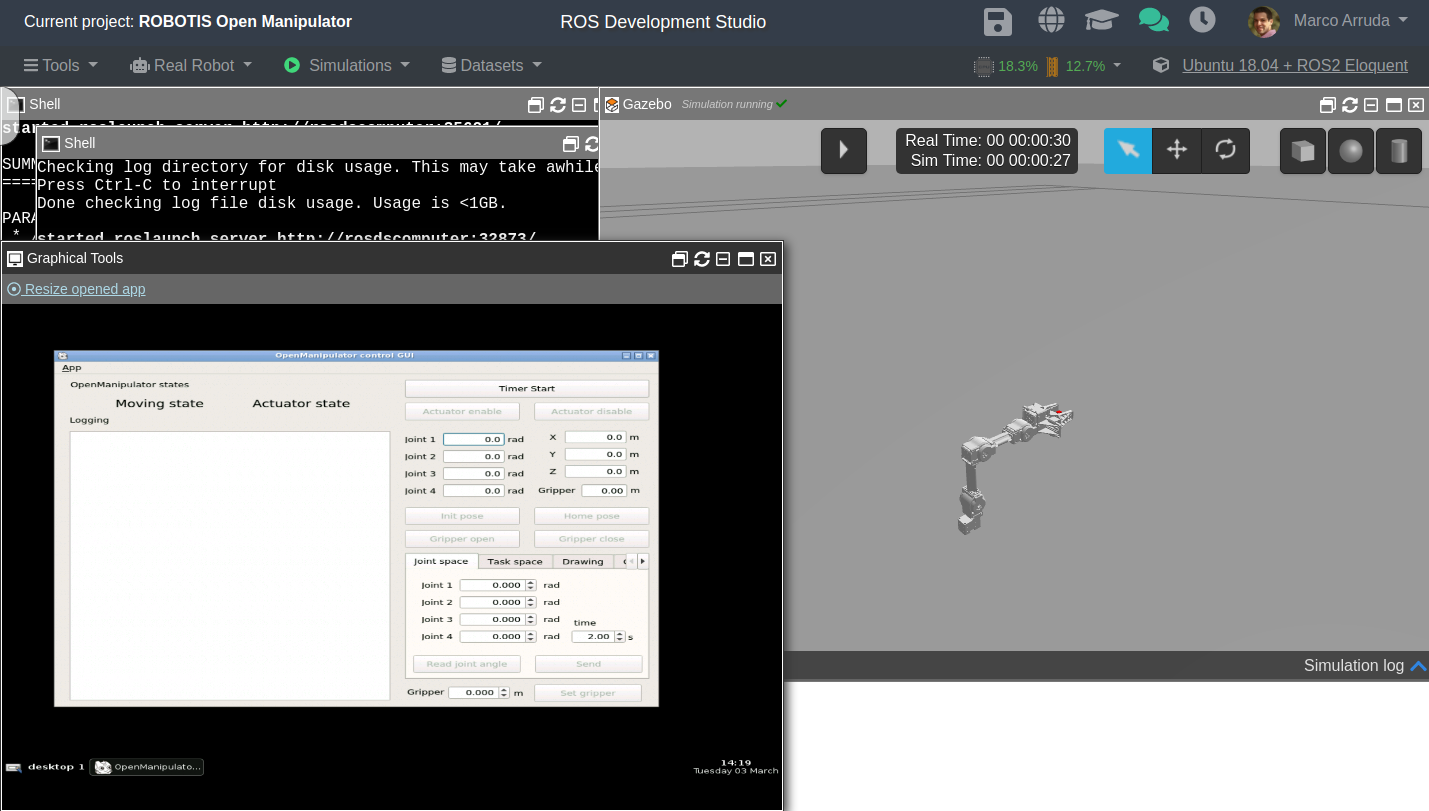
Demonstration
Before pressing the play button of the simulation, run the controllers in the simulation mode:
In this post we are going to setup the simulation of the robot OpenMANIPULATOR-X from Robotis company. All the steps were based on their official documents
Let’s start creating a new ROSJect, we are going to use Ubuntu 18.04 + ROS2 Eloquent, which is also a ROS 1 Melodic environment.
Configuring environment
First we are going to configure our environment for the simulation. Let’s change the $ROS_PACKAGE_PATH in order to avoid the public simulations available in ROSDS.
Let’s recompile the simulation_ws on the folder /home/user/simulation_ws.
After that, get one folder up and re-compile the simulation_ws workspace.
user:~/simulation_ws/src$ cd ..
user:~/simulation_ws$ catkin_make
You must be ready to launch the simulation at this point!
Launching the simulation
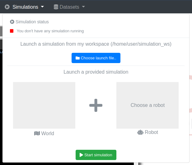
Let’s go on the ROSDS way of launching simulations. Open the simulation menu and press Choose launch file..
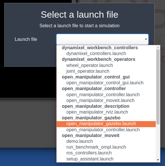
Choose the file open_manipulator_gazebo.launch from the package open_manipulator_gazebo
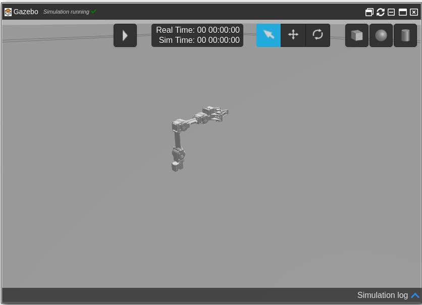
Press Start simulation and the web gazebo client must open the simulation:
Great! Let’s play with it a little bit!
Controllers and GUI Operator
With the simulation ready, let’s start two other programs using the shell.
In a first web shell, shell 1, launch the controllers for gazebo simulator. At this moment, we are telling ROS it’s not a real robot, but a simulated one:
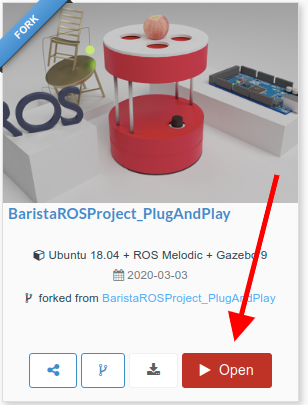
In order to see the simulation, you have to click on the ROSject link (http://www.rosject.io/l/ded2912/) to get a copy of the ROSject. You can now open the ROSject by clicking on the Open ROSject button.
Open ROSject – Barista Robot
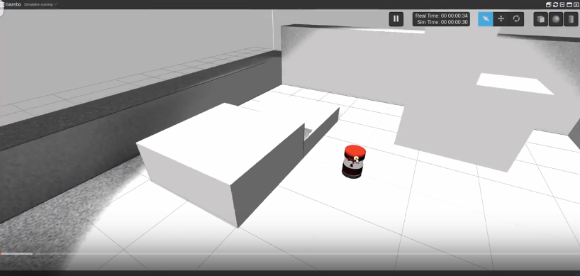
Launching the simulation
With the ROSject open, you can launch the simulation by clicking Simulation, then Choose Launch File. Then you select the main_simple.launch file from the barista_gazebo package.
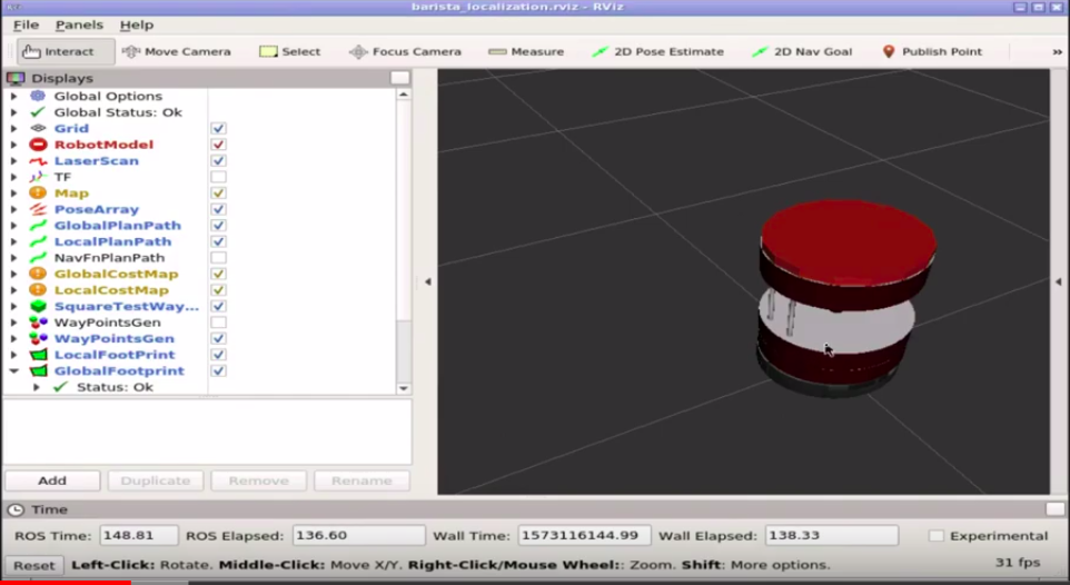
If everything went ok, you should now have the simulation like in the image below:
Barista Robot in ROSDS
The launch file we just selected can be found on ~/simulation_ws/src/barista/barista_gazebo/launch/main_simple.launch and has the following content:
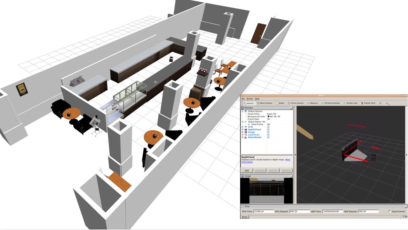
As we can see in the launch file, it spawns the robot and opens RViz (Robot Visualization). You can see RViz by opening the Graphical Tools (Tools -> Graphical Tools).
Barista robot in RViz, in ROSDS
Where is the Barista robot defined
If you look at the launch file mentioned earlier, you can see that we use the put_robot_in_world.launch file to spawn the robot. The content of the file is:
We are not going to explain this file in detail because it will take us a long time. If you need further understanding of URDF files, we highly recommend the URDF for Robot Modeling course on Robot Ignite Academy.
In this file, we essentially load the barista_hexagons_asus_xtion_pro.urdf.xacro file located on the ~/simulation_ws/src/barista/barista_description/urdf/barista/ folder.
At the end of that file we can see that we basically spawn the robot and load the sensors:
You can see that this topic alone publishes too much data.
Since we have to show data in the web app that we are going to create, we use the /diagnostics topic to simulate some elements, like the battery, for example, in the format that the real robot uses.
Showing the Battery status
In the barista_gazebo package, we created the sim_pick_go_return_demo.launch file. There you can see that we spawn the battery_charge_pub.py file, which basically subscribes to the /diagnostics topic and publishes into the /battery_charge topic just basic info about the battery status.
Let’s launch that file to launch the main systems:
If you look at the file sim_pick_go_return_demo.launch we mentioned earlier, in that file we are launching the navigation system, more specifically on the sections shown below:
<!-- Start the navigation systems -->
  <include file="$(find costa_robot)/launch/localization_demo.launch">
    <arg name="map_name" value="simple10x10"/>
    <arg name="real_barista" value="false"/>
  </include>
and
 <!-- We start the waypoint generator to be able to reset tables on the fly -->
  <node pkg="ros_waypoint_generator"
          type="ros_waypoint_generator"
          name="ros_waypoint_generator_node">
    </node>
To start creating the map, please consider reloading the simulation (Simulations -> Change Simulation -> Choose Launch file -> main_simple.launch).
The files related to mapping can be found on the costa_robot package. There you can find the following files:
gmapping_demo.launch
localization_demo.launch
save_map.launch
start_mapserver.launch
To create a map, after making sure the simulation is already running, we run the following:
roslaunch costa_robot gmapping_demo.launch
Now we have the lasers so that we can create the map. To see the lasers, please check RViz using Tools -> Graphical Tools.
You can now move the robot around by running the command below in a new shell (Tools -> Shell), to generate the map:
This saves the current location of the robot as HOME. We can now move the robot around and save the new location. To move the robot around, remember that we use:
Great, so far we know how to start the map, start the localization and save the waypoints.
Youtube video
It may happen that you couldn’t reproduce some of the steps mentioned here. If this is the case, remember that we have the live version of this post on YouTube. Also, if you liked the content, please consider subscribing to our youtube channel. We are publishing new content ~every day.